
In Part 1 of this series, I briefly explained the Elo rating system along with the two key parameters involved. In Part 2, I described how a Bayesian model could be setup to estimate the Elo parameters and the Elo ratings of teams. In this post, I discuss how we can use the model and simulations to estimate the win probabilities of future matches, including the tournament outcome. I assume that the you are familiar with the notations I have used in Part 1 and 2 and hence, will not explain it again here. The source code for this work can be found here.
Estimating the win probabilities for the next round
Assume we want to simulate an outcome for a match between team $A$ and $B$ for round $n+1$. First, let’s fix the Elo parameters $K$ and $\tau$ to some arbitrary values $K^\ast$ and $\tau^\ast$, respectively. Similarly, let’s fix the Elo ratings $r_{A,n}$ and $r_{B,n}$ at $r_{A,n}^\ast$ and $r_{B,n}^\ast$, respectively. For those fixed values, probability of team $A$ winning against team $B$ is given by the parameter of the Bernoulli likelihood function, i.e.
with
\begin{equation} \delta_{A,B,n+1}^\ast = r_{A,n}^\ast - r_{B,n}^\ast. \end{equation}.
We can randomly simulate a match by drawing a sample from $\mathcal{Bern}(\mu_{A,B,n+1}^\ast)$.
So far, we have fixed the Elo parameters and the ratings and by doing so ignored the uncertainty of these parameters. Note that the posterior distribution of these parameters reflect the parameter uncertainty after observing past match outcomes. Therefore, instead of using a fixed set of values for parameters, we could draw many samples from the posterior distributions and use those sample values to simulate match outcomes to account for the uncertainty of these parameters. Conveniently, MCMC samples, after sufficient burn-in/warmup, can be used as draws from the posterior. The proportion of simulated matches that team $A$ won against team $B$ is an approximation of team $A$’s win probability.
Assume I have $M$ draws from the (joint) posterior distribution. I use the superscript notation to indicate the sample number. For example, $\tau^{(m)}$ denote the MCMC sample for $\tau$. Let $W_{A,B,n+1}^{(m)}$ denote the simulated match outcome (for round $n+1$) drawn from the Bernoulli distribution with parameter $\mu_{A,B,n+1}^{(m)}$, i.e.
where $\mu_{A,B,n+1}^{(m)}$ is calculated using $\tau^{(m)}, r_{A,n}^{(m)}$ and $r_{B,n}^{(m)}$.
Posterior probability of team $A$ winning against $B$ in round $n+1$ can be approximated as $\frac{1}{M}\sum_{m=1}^M W_{A,B,n+1}^{(m)}$.
Looking under the hood
Why is $\frac{1}{M}\sum_{m=1}^M W_{A,B,n+1}^{(m)}$ an approximation to team $A$’s winning probability and what does it got to do with Bayes? Let me explain.
Formally, what we are after is the posterior predictive distribution for the outcome of the next match. In other words, what probability do we assign to the outcome of a future match, after observing the actual outcomes of rounds 1 to $n$. Let $\mathbf{W}_{A,B,n}$ denote a vector of match outcomes of all the past matches up to and including round $n$. Then, the posterior predictive distribution can be approximated as follows.
First equality follows from Chapman-Kolmogorov equation. Second equality is due to the conditional probability formula. Note the term $p(\tau,r_{A,n},r_{B,n}|\mathbf{W}_{A,B,n})$ is the joint posterior distribution of (some of) the parameters from the Elo model. Third line follows by using a Monte Carlo approximation to the integral using the MCMC samples which approximate the draws from the posterior distribution.
Is the model output well calibrated?
One of the most desirable properties of a model is to have well calibrated probabilities. If I have to pick one metric to evaluate a model, it would definitely be the calibration check. What I mean by well calibrated probabilities is, for example, if the model predicts a team wins with 80% probability, then of all the times such predictions are made, the team should win approximately 80% of the time. This should hold not just for 80%, but for all probabilities.
To assess the calibration, I considered all the matches from round 5 to 22, which consists of 153 matches. Each round’s predictions were made using the the model trained with data up to and including the previous round. I binned the winning probabilities of the first team into bins of width 10% (i.e. 0 to .1, .1 to .2, … ,.9 to 1). For each bin, I calculated the average prediction probability and the fraction of times the first team actually won. These points were then plotted. A “perfect” model would have all the points lying on the $y=x$ line. For comparison purposes, I trained the model with all the data including round 22, and retrospectively predicted the previous rounds. The graph below shows the output of the calibration assessment.
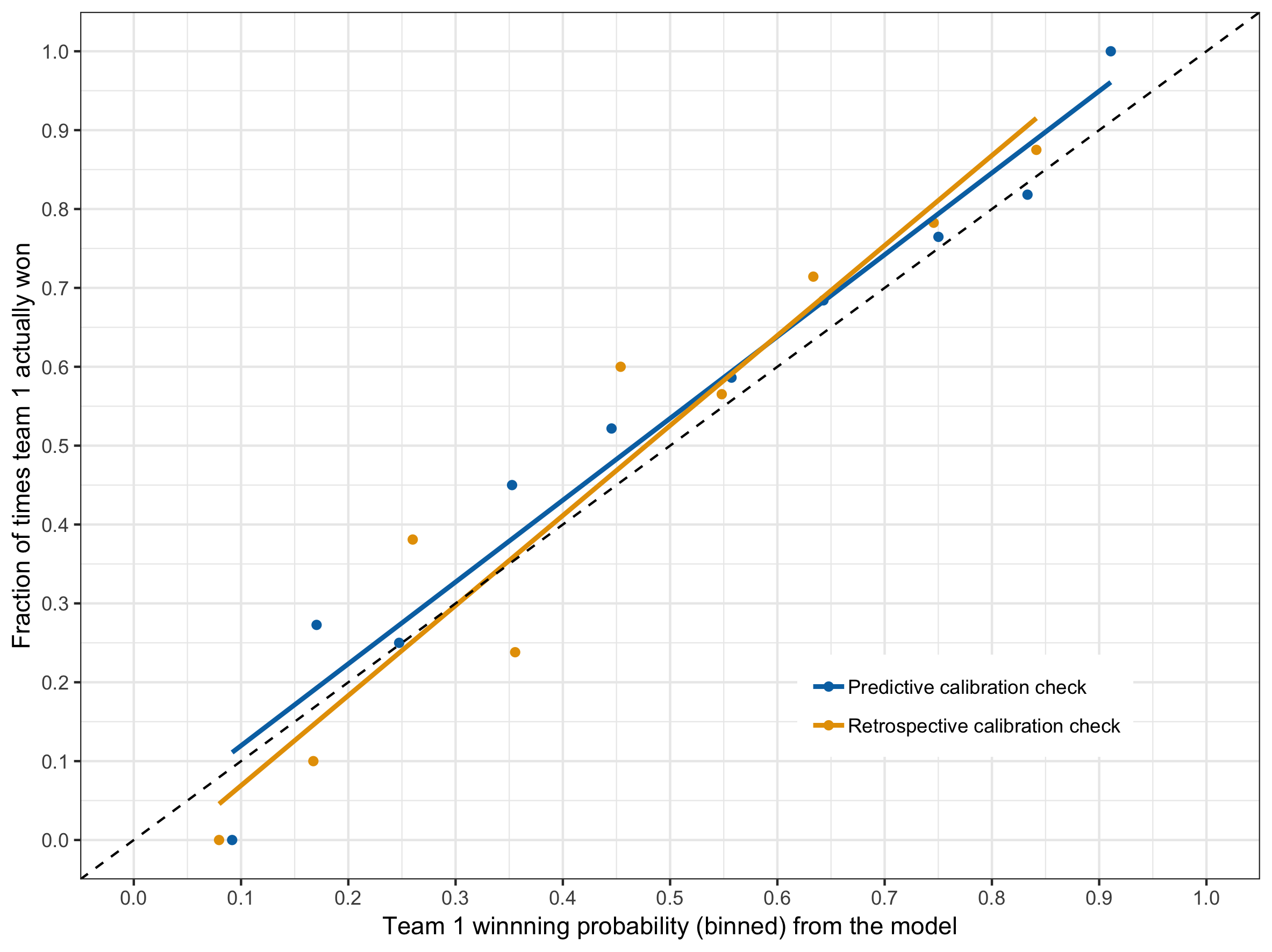
Based on the above results, I’m reasonably satisfied with the calibration.
Model evaluation against some standard metrics
I have tabulated some of the standard model evaluation metrics based on the match outcomes for rounds 5 through to 22. Similar to the calibration check, I’ve calculated the metrics in both the foresight (predictive) and hindsight (retrospective) directions.
| Metric | Predictive | Retrospective |
|---|---|---|
| Accuracy | 0.65 | 0.67 |
| AUC | 0.72 | 0.75 |
| Precision | 0.69 | 0.71 |
| Recall | 0.65 | 0.65 |
For accuracy, precision and recall calculations, the model predictions were converted to binary form using a threshold of 0.5. A positive thing to note is that predictive and retrospective metrics are similar. Comparing predictive and retrospective metrics is analogous to comparing testing and training performance in machine learning.
Simulating matches beyond the immediate round
In order to workout the probabilities of winning the premiership title, we need to simulate future matches not just for the next round, but until a team wins the premiership. If we can simulate these virtual tournaments many times, then the proportion of times a given team ends up winning the premiership is an approximation for that team’s probability of winning the tournament. The power and flexibility of Monte Carlo simulations is that the same method can be used to find probabilities of other events such as a team making the top 8, semi finals or preliminary finals, etc.
Our parameter space for which MCMC samples are drawn from is multidimensional. That is, after $n$ (physical) rounds of matches, the parameters in our model for which the inference is performed include, $K$, $\tau$ and Elo rating for each team after each round (up to and including round $n$). It should be noted that a single sample from the MCMC chain gives a realisation for each of these parameters. For each MCMC sample, I created a trajectory of simulated outcomes for future matches leading up to the premiership title. The important thing to note is that outcomes of the simulated matches are used to update the Elo ratings for future rounds according to the Elo update formula, which I discussed in Part 1 and 2.
There is a subtle point that I wish to emphasise here. Because I update the future Elo ratings based on the simulated outcomes (as opposed to actual match results), I implicitly assume that the future Elo rating changes are purely based on current Elo ratings and the stochastic nature of the dynamics induced by the Elo framework. In other words, factors such as future changes in team morale or injuries which may have an effect on team performance, are not captured because the Elo rating updates for the future rounds are based on simulated match outcomes instead of actual match outcomes. Another way of saying this is, I ignore the possibility of genuine new skill acquisitions (or depletion) that may happen in future.
The MCMC for parameter estimation and future match simulation were both handled via Stan. Though I had some limited experience with Stan before, this was the first time I used it extensively. Beyond round 23, only eight teams progress to the finals series. Here, the future schedule is not fixed and depends on the outcome of the previous matches. Because Stan is a probabilisitic programming language and not a general purpose language like Python, there was a bit of a learning curve involved in figuring out how to implement the “AFL final eight system” in Stan.
Probabilities of each team reaching a milestone in the finals series
The milestones considered are
- a team making it to the final 8
- a team making it to the the semi final
- a team making it to the the preliminary final
- a team making it to the grand final
- a team winning the premiership.
Below I present the probabilities evaluated at 2 different times (after round 15 and 22) as the season progressed. Rows are sorted in the descending order of premiership winning probability and the probabilities are rounded to the to nearest two decimal points.
Final series probabilities evaluated after round 15
| Team | Final 8 | Semi final 4 | Preliminary final 4 | Grand final 2 | Premiership |
|---|---|---|---|---|---|
| Richmond | 1.00 | 0.42 | 0.79 | 0.43 | 0.24 |
| Sydney | 0.94 | 0.47 | 0.59 | 0.31 | 0.16 |
| Port Adelaide | 0.96 | 0.48 | 0.58 | 0.31 | 0.15 |
| Collingwood | 0.93 | 0.47 | 0.53 | 0.27 | 0.14 |
| West Coast | 0.92 | 0.48 | 0.48 | 0.22 | 0.10 |
| GWS | 0.56 | 0.29 | 0.19 | 0.09 | 0.04 |
| Geelong | 0.58 | 0.29 | 0.19 | 0.08 | 0.04 |
| Hawthorn | 0.60 | 0.30 | 0.17 | 0.08 | 0.04 |
| North Melbourne | 0.57 | 0.29 | 0.17 | 0.08 | 0.03 |
| Melbourne | 0.55 | 0.27 | 0.17 | 0.07 | 0.03 |
| Essendon | 0.19 | 0.11 | 0.07 | 0.04 | 0.02 |
| Adelaide | 0.17 | 0.09 | 0.05 | 0.02 | 0.01 |
| Fremantle | 0.03 | 0.02 | 0.01 | 0.00 | 0.00 |
| Western Bulldogs | 0.00 | 0.00 | 0.00 | 0.00 | 0.00 |
| St Kilda | 0.00 | 0.00 | 0.00 | 0.00 | 0.00 |
| Brisbane Lions | 0.00 | 0.00 | 0.00 | 0.00 | 0.00 |
| Carlton | 0.00 | 0.00 | 0.00 | 0.00 | 0.00 |
| Gold Coast | 0.00 | 0.00 | 0.00 | 0.00 | 0.00 |
Final series probabilities evaluated after round 22
| Team | Final 8 | Semi final 4 | Preliminary final 4 | Grand final 2 | Premiership |
|---|---|---|---|---|---|
| Richmond | 1.00 | 0.37 | 0.86 | 0.55 | 0.34 |
| West Coast | 1.00 | 0.51 | 0.73 | 0.33 | 0.15 |
| Sydney | 1.00 | 0.57 | 0.54 | 0.27 | 0.13 |
| Collingwood | 1.00 | 0.51 | 0.62 | 0.27 | 0.12 |
| Hawthorn | 1.00 | 0.57 | 0.48 | 0.23 | 0.11 |
| GWS | 1.00 | 0.54 | 0.32 | 0.15 | 0.07 |
| Melbourne | 1.00 | 0.50 | 0.27 | 0.12 | 0.05 |
| Geelong | 0.93 | 0.40 | 0.17 | 0.08 | 0.03 |
| Port Adelaide | 0.07 | 0.03 | 0.01 | 0.01 | 0.00 |
| Adelaide | 0.00 | 0.00 | 0.00 | 0.00 | 0.00 |
| Brisbane Lions | 0.00 | 0.00 | 0.00 | 0.00 | 0.00 |
| Carlton | 0.00 | 0.00 | 0.00 | 0.00 | 0.00 |
| Essendon | 0.00 | 0.00 | 0.00 | 0.00 | 0.00 |
| Fremantle | 0.00 | 0.00 | 0.00 | 0.00 | 0.00 |
| Gold Coast | 0.00 | 0.00 | 0.00 | 0.00 | 0.00 |
| North Melbourne | 0.00 | 0.00 | 0.00 | 0.00 | 0.00 |
| St Kilda | 0.00 | 0.00 | 0.00 | 0.00 | 0.00 |
| Western Bulldogs | 0.00 | 0.00 | 0.00 | 0.00 | 0.00 |
Note that except for the last column (premiership), other columns do not need to add up to 1 as events are not necessarily mutually exclusive (eg. team A making it to the final 8 does not mean team B cannot). After round 22, 7 positions out of 8 are already occupied and there was significant chance of Geelong securing the last spot. Compare this with the probabilities after round 15, where only 1 position (Richmond) is guaranteed. These results were obtained by running many (40,000) virtual tournaments. The main point I like to emphasise here is that Bayesian framework, along with simulations, gives a very flexible and powerful platform for modellers.
What’s next?
There are many enhancement opportunities for the current implementation of the Bayesian Elo model. Adjusting the Elo update formula to account for home field advantage is one of them. Home field advantage is the apparent advantage a team enjoys when a match is played at its home ground. For some discussion on what is driving the home field advantage, please refer to the book “Scorecasting”. The Elo update formula can be adjusted so that when a team records a win in its home ground, the increment in the Elo rating is lesser than the same team recording a win away from the home ground.
Margin of victory adjustments, details of which I discussed in Part 1 of this series, is not used in the current implementation. This adjustment treats a win by just 1 point different to a win by a significant margin. The challenge of using that adjustment is with simulating the future matches. This is because, with margin of victory adjustment, Elo rating update would require simulated team scores instead of just win/lose outcomes. Predicting team scores is more challenging than predicting the binary outcome of a match.
Using data over multiple seasons, a multilevel model can be fitted to capture year-to-year fluctuations in the Elo parameters. This may also help with adding some additional regularisation for the model fit.