
In Part 1 of this three-part series, I presented an introduction to the Elo rating system. In this post, I describe the specifics of the Bayesian model used to infer the Elo parameters $K$ and $\tau$. I also illustrate how the parameter uncertainty is reflected in Elo ratings by showing the posterior distribution of the ratings for two teams (St. Kilda and West Coast Eagles) as the season progressed. Instead of a single point estimate for a team’s Elo rating, we can get a more informative view by looking at plausible values of Elo expressed as a probability distribution. This is a precursor for the final piece of the puzzle, covered in the Part 3, where I estimate the win probabilities for future matches, including the Premiership title. The source code for this work can be found here.
Modelling
Prior distributions
The model specified here is extremely simple. First, I treat the Elo parameters $K$ and $\tau$ as random parameters and assign somewhat weakly informative Normal distributions as follows;
where $\mathcal{N}(\mu,\sigma^2)$ denotes a Normal distribution with mean $\mu$ and standard deviation $\sigma$. To understand why the above prior choices are weakly informative, notice that $K$ could take a value in the range of 0 to 300 with approximately 95% probability, easily covering the typical $K$ values used in sports. Similarly, the approximate 95% interval for $\tau$ is (200,600).
Let $r_{i,n}$ denote the Elo rating of team $i$ after round $n$. The Elo rating at the beginning of the season is denoted by $r_{i,0}$. What prior should I assign to $r_{i,0}$? One option would be to look at the past seasons of the teams and assign priors accordingly, perhaps, with some allowance for regression to the mean. But, I take a simple approach by ignoring additional data and assume all the teams’s initial Elo ratings are independent and identically distributed, i.e.
\begin{equation} r_{i,0} \sim \mathcal{N}(1500,100^2). \end{equation}
Likelihood
Let $W_{i,j,n}$ denote the outcome of a match between team $i$ and $j$ encountered in round $n$.
In the above equation, I do not distinguish between a loss and a tie for convenience.
Now let’s define $\delta_{i,j,n}$ as \begin{equation} \delta_{i,j,n} = r_{i,n-1} - r_{j,n-1}. \end{equation}.
To form the likelihood function, I model $ W(i,j,n)$ as a Bernoulli trial with parameter $\mu_{i,j,n}$ where
Once the outcome of the round $n$ match is available, Elo ratings are updated according to
where
Using the the actual match outcomes, we can approximate the posterior distributions of the Elo parameters $K$, $\tau$ and the team ratings $r_{i,n}$ using Markov Chain Monte Carlo (MCMC). I used Stan to implement this model.
Results
After fitting the model with the match outcomes up to and including round 23, the posterior distributions for $K$ and $\tau$ are shown below. The solid lines represent the posterior distribution while the dashed lines represent the prior.
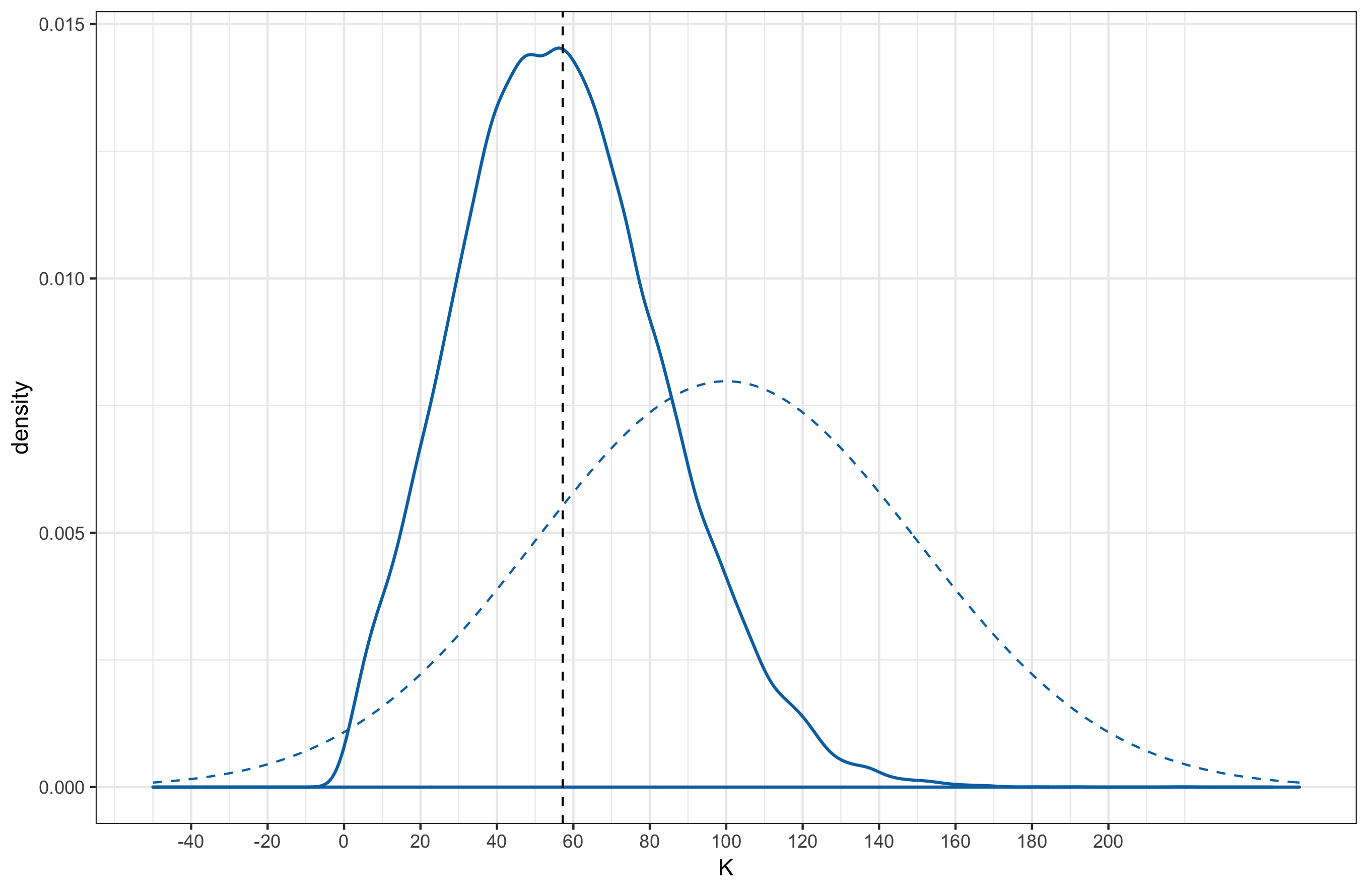
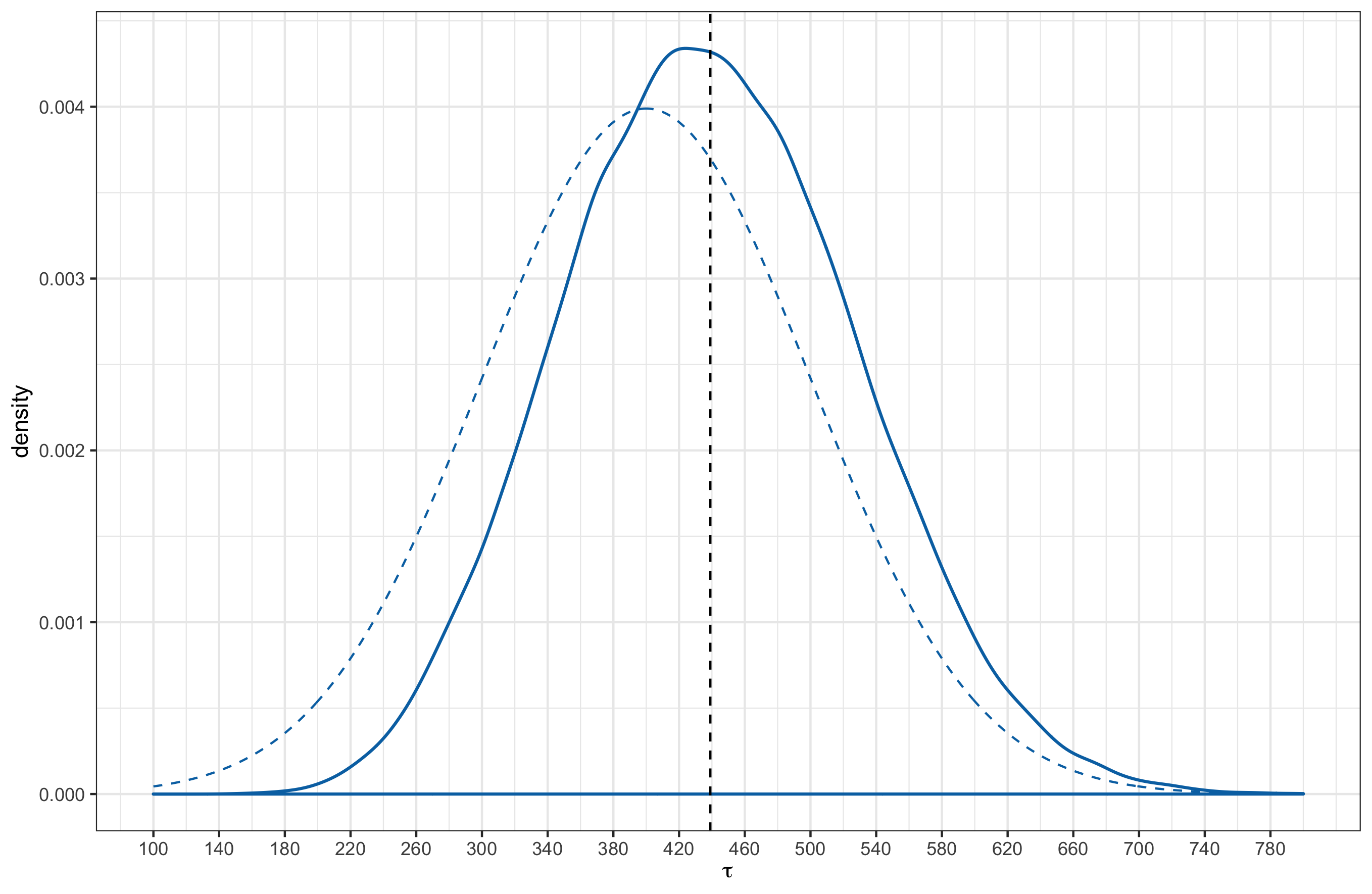
Posterior distributions were approximated from 4 parallel Markov Chains, each of length 10,000 (20,000 samples were drawn from each chain, but the first 10,000 was discarded as warmup).
Posterior point estimates (derived from MCMC samples) for the Elo parameters are shown in the following table along with the standard deviation.
| parameter | posterior mean | posterior standard deviation |
|---|---|---|
| $K$ | 57.22 | 26.77 |
| $\tau$ | 439.04 | 89.06 |
How sensitive is the posterior to different choices of prior distributions?
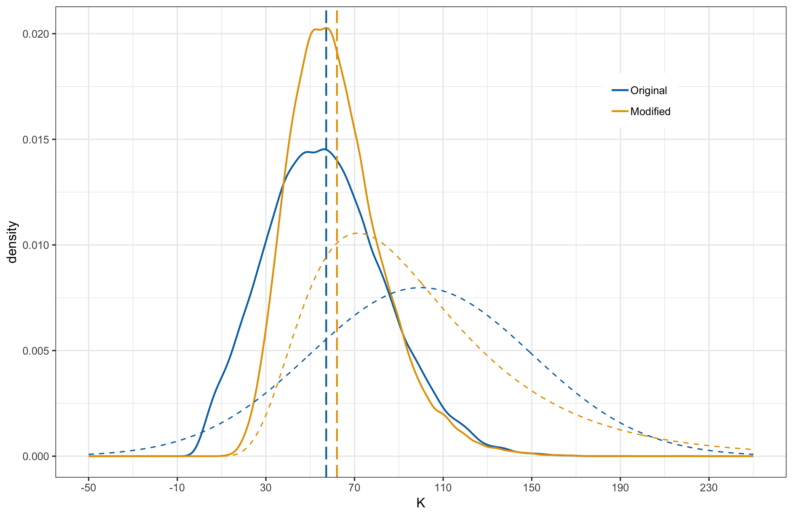
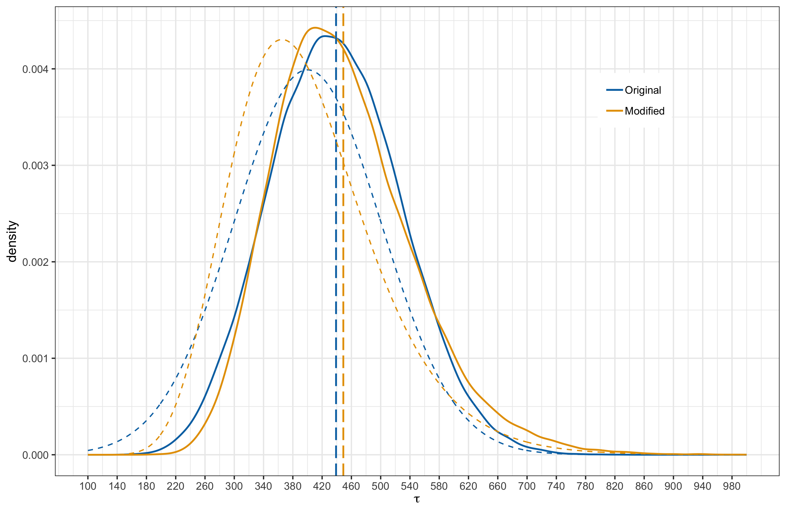
Prior distribution and likelihood are modelling assumptions and it is a good practice to check how sensitive the model outputs are to these assumptions. This is known as sensitivity analysis. Here, I will alter the prior distributions of $K$ and $\tau$ and compare the effect on the posterior distributions. Sensitivity to the prior is not necessarily a bad thing; after all, the prior distribution gives an opportunity to feed domain knowledge to the model. But we need to be extra skeptical of models that are highly sensitive to small changes in the prior, or at-least be aware of it.
Recall that our original prior assignments for $K$ and $\tau$ are and , respectively. In this analysis I consider 3 alternative specifications.
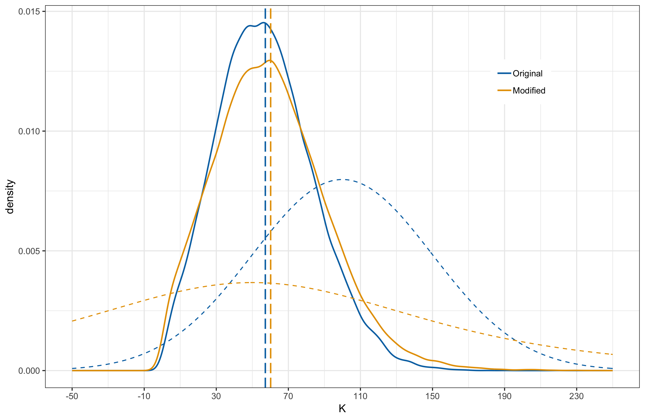
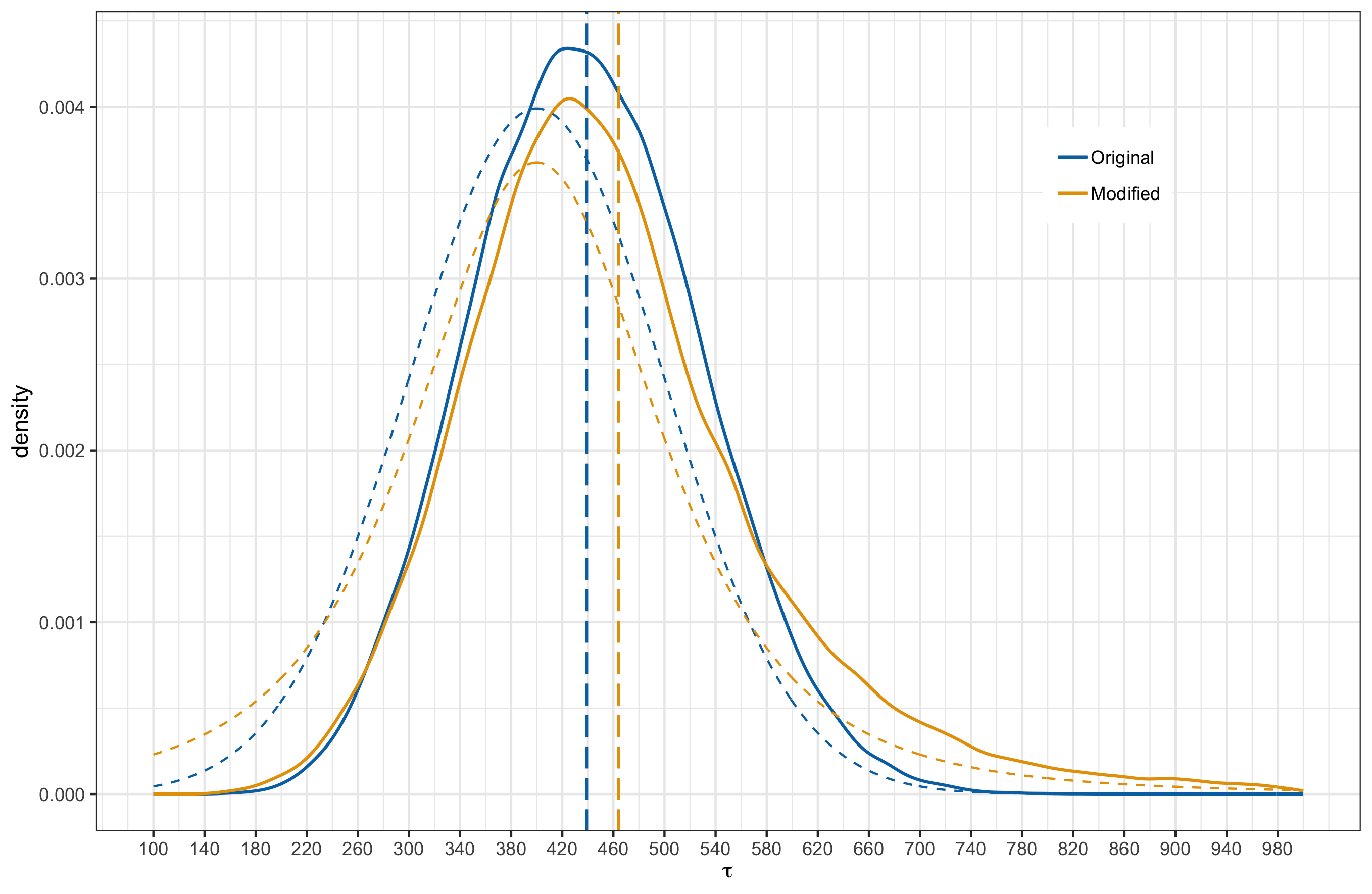
- Case 1: Lognormal distribution with the same mean and standard deviation as the original prior.
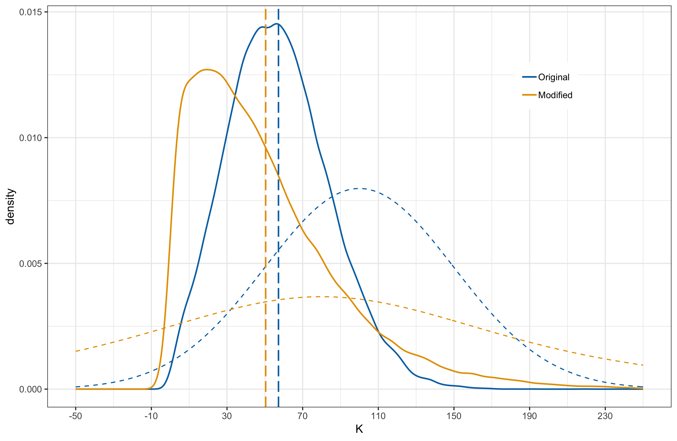
- Case 2: student-t distribution with degree of freedom set to 3 and mean matching the original prior specification.
- Case 3: student-t distribution with degree of freedom set to 3 and mean parameter shifted from that of the original but scaling parameter set to have heavier tails.
Below, I provide plots comparing the original and new posterior induced by the alternative priors. I have overlayed the prior distributions as dashed curves and the vertical lines mark the posterior means.
| case 1: $K$ | case 1: $\tau$ |
|---|---|
 |
 |
| case 2: $K$ | case 2: $\tau$ |
|---|---|
 |
 |
| case 3: $K$ | case 3: $\tau$ |
|---|---|
 |
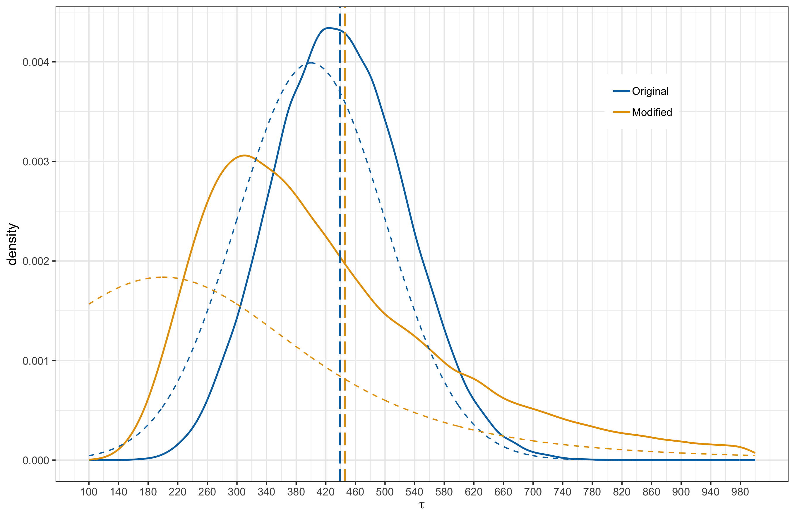 |
In all cases, the posterior means remain close to each other. When comparing the distribution shapes, case 2 results in the least shift from the original posterior. Most noticeable shift occurs in case 3 where we have shifted the mean in the prior and made the tails heavier. This is something to be a bit weary about. Also of interest is the fact that even under case 3, where the modified prior for $K$ has significant probability mass to the left of 0, the posterior does not have probability mass over negative $K$ values. In other words, model is indicating that negative $K$ values are strongly inconsistent with the observed data.
Team Elo ratings as the season progressed
Note that we assigned a $\mathcal{N}(1500,100^2)$ prior for each team’s Elo rating at the beginning of the season (i.e round = 0). This prior distribution for the Elo ratings for round 0, together with the Elo update formula, implicitly induce prior distributions for Elo ratings for all rounds. The MCMC samples from the fitted model can be used to approximate the posterior distributions for Elo ratings, after each round, for any team. Below, I plot this for two teams, St Kilda and West Coast Eagles. West Coast Eagles turned out to be the eventual winners of the tournament, while St. Kilda did not have a good season. In the below graphs, density plots for each round are stacked vertically. The dashed vertical lines indicate the base Elo rating of 1500 (mean of the prior assigned to initial Elo ratings).

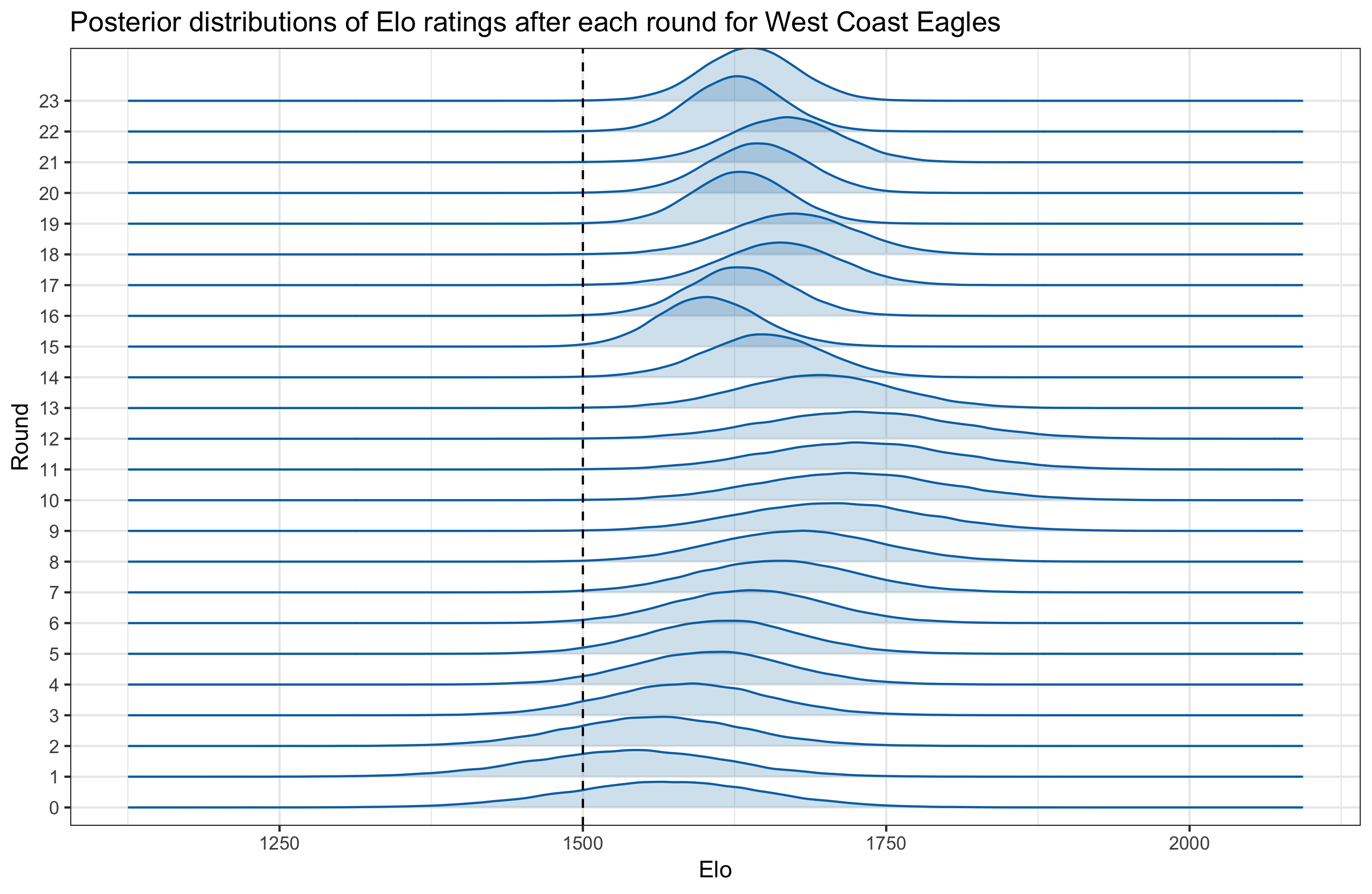
Contrast the movement of Elo ratings for the two teams. St Kilda started off the season with an average Elo rating of 1434 and drifted to 1302 by the end of round 23. On the other hand, West Coast Eagles started the season with an average rating of 1567 and increased it to 1638 by round 23.
Lets take a step back to reflect on what these posterior distributions mean. Under Bayesian inference, posterior distribution gives the correct answer to the question, “For a given model specification, which set of parameters are more plausible to result in the observed data?”. Embedded in the question are our assumptions on how the world behaves (specified by likelihood and prior) and it may not reflect the reality. This difference between modelling assumptions and reality is nicely explained in the book “Statistical Rethinking” by Richard McElreath. He uses the words “small world” and “large world” to explain this concept. Small world represents the assumptions and the self contained logic that we assume the world operates by while “large world” represents the true nature. Bayesian inference gives the optimum answer to the questions posed under small world assumptions, but it does not a guarantee that the answers are correct under large world assumptions. It is up to the modeller to reason out and come up with proper questions (in the form of likelihood and prior) to be answered by Bayesian inference. To relate this to our current exercise, I should be questioning the validity of the model, for example, “is it reasonable to assume that the probability of a team A winning against team B is related to a logistic function of the difference of current Elo ratings?”, etc. In this series of posts, I am not attempting to validate the small world assumptions, but instead focus on finding the best possible answers to the questions posed under such assumptions.
In the 3rd and final part of the series, I will go into the details of how we can simulate the remainder of the tournament and use these simulation results to approximate the probability of each team making it to the finals series or winning the Premiership title, etc.